Identifying Salient Issues in Interstate Conflicts Using Topic Modeling

Data preparation

The process starts with the reading of the text data. The texts’ length affects the results of topic modeling. Therefore, for very short texts (e.g., Twitter posts) or very long texts (e.g., books), it is advisable to concatenate/split single documents to get longer/shorter text units. By performing a qualitative review of the results, we can determine if these approaches leads to more interpretable topics. After a brief review of my results, I see no reason to use these approaches for analyzing the articles at hand.

For text preprocessing, I stem words and convert letters to lowercase. I also remove special characters and stop words (i.e., function words that have relational rather than substantive meaning). Stop words are problematic because they appear as “noise” in the estimated topics generated by the LDA model.

Thereafter, I create a Document-Term-Matrix (DTM) of the corpus. This matrix describes the frequency of terms that occur in a text collection, where the rows correspond to texts in the collection and the columns correspond to terms. Thereby, I only consider terms that occur with a minimum frequency of 15 times within the corpus. This is primarily to speed up the model calculation.

Calculate topic model

The calculation of topic models aims to determine the proportional composition of a fixed number of topics in the documents of a collection. For parameterized models such as LDA, the number of topics (K) is the most important parameter to define in advance. It is worth to experiment with different parameters to find the most suitable parameters for your own analytical needs. If K is too small, the collection will be split into a few very general topics. If K is too large, the collection will be divided into far too many topics, where some overlap and others are almost impossible to interpret.

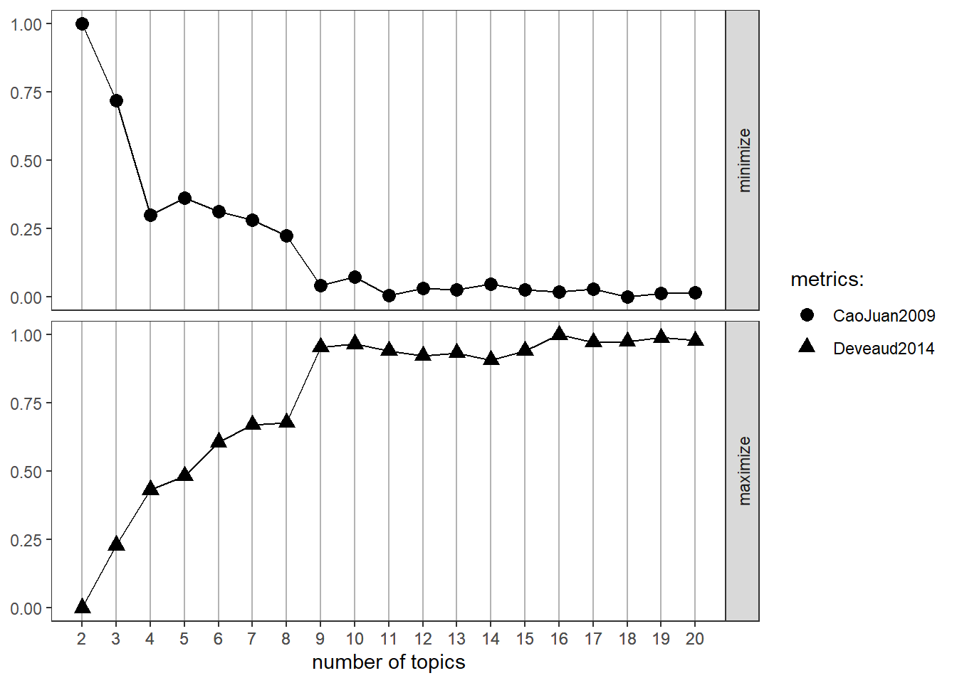
One procedure for deciding on a specific topic number is the usage of the ldatuning package which uses some metrics to find optimal number of topics for LDA models (Nikita & Chaney, 2020). This approach can be useful when the number of topics is not theoretically motivated or based on a qualitative data inspection. For illustrative purposes, I use the two methods CaoJuan2009 and Griffith2004. But it is recommendable to inspect the results of the four metrics available (Griffiths2004, CaoJuan2009, Arun2010, and Deveaud2014). Furthermore, I choose a thematic resolution of 20 topics. In contrast to a resolution of 100 or more, this number of topics can be easily evaluated qualitatively. We can now plot the results. The best number of topics shows high values for Griffith2004 and low values for CaoJuan2009. Optimally, several methods should converge and show peaks and drops respectively for a certain number of topics. The inference of topic models can take a long time depending on the vocabulary size, the collection size, and K. This calculation takes several minutes. If it takes too long, we can reduce the vocabulary in the DTM by increasing the minimum frequency. Looking at the graphical representation (Fig. 2), we can conclude that the optimal number of topics is 16. We use this number to compute the LDA model.

Fig. 2 Finding the optimal number of topics

The model calculation results in two probability distributions. The first result, called theta here, shows the distribution of topics within each document. The second outcome, named beta, shows the probability that a word appears in a specific topic.

Depending on our research goals, we might be interested in a more pointed or a more even distribution of topics in the model. The distribution of topics within a document can be controlled with the alpha parameter of the model. In the first model calculation the alpha parameter was automatically estimated in order to fit the data (highest overall probability of the model). If we now increase the alpha value, we get a more even distribution of topics within a document. If we decrease the alpha value, the inference process distributes the probability mass on a few topics for each document.

In the following case, I am interested in the most salient topics within the interstate relations. Therefore, I decide for a more pointed distribution of topics and change the alpha parameter to a lower value to create a second model. To see how this affects the distribution, I compare the topic distribution within three sample documents according to both models. For the next steps, we give the topics more descriptive names by concatenating the five most likely terms of each topic to a string that represents a pseudo-name for each topic. In the first model, all three documents show at least a small percentage of each topic. In the second model, all three documents only show a few dominant topics (Fig. 3).

Fig. 3 Effect of a modified alpha parameter on topic distribution

Overview of topic related terms

Relying on the results of the second model, I create a word cloud for each topic which gives a quick visual overview on the related terms. For the sake of clarity, I only select the 40 terms with the highest probability to appear in a given topic (Fig. 4). At first glance, relying on my case knowledge, a large number of the identified topics appear to be valid. But some topics seem either too general (e.g., peopl_year_day_time_live) or entirely irrelevant (e.g., iraq_weapon_nuclear_offici_american).

Fig. 4 Illustration of topic-related terms

Topics over time

In the next step, I provide an overview of the occurrence of topics within the articles over time. For this purpose, I determine the average share of topics in the annual news coverage and visualize these aggregated topic proportions using a bar plot (Fig. 5). I can now use this bar plot to identify topics related to interstate conflict events.

Fig. 5 Topics over time

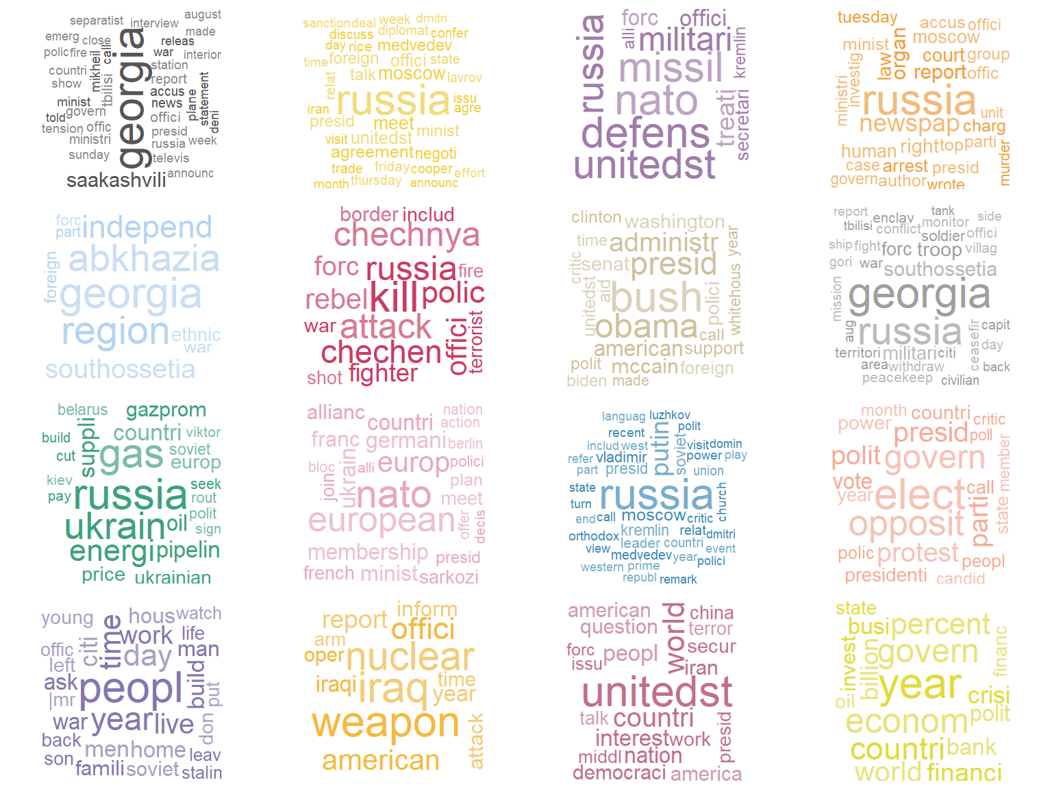
By comparing the intensity trends of conflict actions with the aggregated topic proportions, we see that topics around Russian energy supplies as well as legal procedures clearly dominate the year 2006. The breakaway regions South Ossetia and Abkhazia as well as the Georgian NATO membership are the most important topics in the year 2008. However, some topics are very nebulous and require further background information.

In summary, we can conclude that topic modeling is a very helpful approach for detecting salient issues in interstate conflicts from scratch. We can use these results to look at the occurrence of topics over time. Thereby, we should bear in mind that the representation of topics depends on the composition of the underlying text collection.

Furthermore, we can use the topic model for thematic filtering of a text collection based on the topic probabilities for each document. By investigating these thematic text collections, we can use information retrieval approaches (e.g., the implicit network approach) to identify relations between these topics and other potential entities (e.g., state leaders, dates, and locations) and to dig deeper into the context (see Cujai (2022) for further details).

References

The presented conflict trends are drawn from an adjusted version of the ICEWS data set which only contains interstate conflict actions. The data selection process reveals limited availability of data on interstate conflict events explaining the shortened investigation period. For more information on the selection process, see Cujai, S. (2021): Determination of Interstate Conflict Trends with ICEWS. https://tinyurl.com/2dyh67su↩︎